
⚡Forecasting Brazilian Electricity Demand using TimeGPT
This study investigates the application of foundational models for forecasting the Brazilian hourly electricity load curve. Accurate and reliable electricity demand forecasts are critical for operational planning, resource allocation, and maintaining grid stability within complex energy systems. Given the increasing integration of renewable energy sources and the dynamic nature of energy consumption patterns, advanced forecasting methodologies are essential to address the inherent uncertainties in electricity markets.
In this notebook, we present a comprehensive demonstration of leveraging TimeGPT, a prominent foundational model, for this demanding forecasting task. The analysis encompasses the entire forecasting workflow, beginning with the acquisition of historical hourly load data from the Brazilian National Electric System Operator (ONS).
Subsequent steps involve rigorous data processing to prepare the dataset for model ingestion, followed by the implementation of both zero-shot and fine-tuned forecasting strategies using TimeGPT. The performance of these models will be critically evaluated using established metrics such as Mean Absolute Error (MAE) and Symmetric Mean Absolute Percentage Error (sMAPE), with a particular focus on understanding the impact of fine-tuning parameters on predictive accuracy across different regional subsystems.
🤖 About Foundation Models and TimeGPT
Foundation models represent a paradigm shift in time series forecasting, leveraging extensive pre-training on diverse datasets to acquire a generalized understanding of temporal dynamics. Unlike traditional models requiring specific training for each time series, these large-scale models exhibit robust zero-shot and few-shot learning capabilities, enabling accurate predictions on unseen data with minimal or no prior fine-tuning. This intrinsic adaptability significantly reduces the computational and data-intensive overhead associated with developing bespoke forecasting solutions.
TimeGPT, developed and maintained by Nixtla, exemplifies a cutting-edge foundational model specifically designed for time series analysis. It capitalizes on its pre-trained knowledge base to forecast future values across various domains, including critical applications such as electricity demand. Its architecture facilitates both immediate inference and performance enhancement through targeted fine-tuning. As a proprietary offering, TimeGPT operates on a subscription-based model.
🔮 Forecasting with TimeGPT
🗃️ Libraries
'''
Installs the `utilsforecast` library,
which provides various utility functions for time series forecasting.
'''
!pip install utilsforecast --quiet

'''
Installs the `nixtla` library, which is used to connect with TimeGPT
'''
!pip install nixtla --quiet

'''
Installs the `mlforecast` library,
which allows the use of various machine learning models
for comparison in time series forecasting.
'''
!pip install mlforecast --quiet
[2K [90m━━━━━━━━━━━━━━━━━━━━━━━━━━━━━━━━━━━━━━━━[0m [32m40.3/40.3 kB[0m [31m801.7 kB/s[0m eta [36m0:00:00[0m
[2K [90m━━━━━━━━━━━━━━━━━━━━━━━━━━━━━━━━━━━━━━━━[0m [32m48.5/48.5 kB[0m [31m1.6 MB/s[0m eta [36m0:00:00[0m
[2K [90m━━━━━━━━━━━━━━━━━━━━━━━━━━━━━━━━━━━━━━━━[0m [32m128.1/128.1 kB[0m [31m3.6 MB/s[0m eta [36m0:00:00[0m
[2K [90m━━━━━━━━━━━━━━━━━━━━━━━━━━━━━━━━━━━━━━━━[0m [32m348.2/348.2 kB[0m [31m11.4 MB/s[0m eta [36m0:00:00[0m
[2K [90m━━━━━━━━━━━━━━━━━━━━━━━━━━━━━━━━━━━━━━━━[0m [32m419.5/419.5 kB[0m [31m20.9 MB/s[0m eta [36m0:00:00[0m
[?25h
# Load libraries for data handling
import numpy as np
import pandas as pd
import matplotlib.pyplot as plt
import matplotlib.dates as mdates
from datetime import datetime

# Import TimeGPT client from nixtla library
from nixtla import NixtlaClient

# Import auxiliary functions for evaluation and plotting from utilsforecast
from utilsforecast.losses import mae, smape
from utilsforecast.evaluation import evaluate
from utilsforecast.plotting import plot_series

# Import prediction intervals, lag transforms, and target transforms from mlforecast
from mlforecast.utils import PredictionIntervals
from mlforecast.lag_transforms import ExpandingMean, RollingMean
from mlforecast.target_transforms import Differences

# Import MLForecast model and LightGBM regressor for comparison
from mlforecast import MLForecast
import lightgbm as lgb

# Import BaseEstimator for custom model implementation
from sklearn.base import BaseEstimator

# Import userdata to retrieve the API key from Colab Secrets
from google.colab import userdata
⚙️ TimeGPT Initial Setup
🔑 Get your API key
Access to the TimeGPT model, being a proprietary service, necessitates an API key. This key serves as an access token, enabling authenticated interaction with the TimeGPT API. Users can generate their API keys through the designated platform.
For enhanced security, it’s best practice to store your API key in a .env file located at the root of your project directory. This prevents the key from being directly exposed in your codebase.
For example, your project structure might look like this:
project_folder/
|---.env
|---my_script.py
Within this Colab environment, the userdata.get function was employed to retrieve the API key.
Another method involves utilizing the python-dotenv package to load key-value pairs from a .env file and set them as environment variables.
🏁 Initializing NixtlaClient
# Instantiate the NixtlaClient...
nixtla_client = NixtlaClient(
    # ...and insert your API key
    api_key= userdata.get('MY_API_KEY')
    )
Use the validate_api_key method of NixtlaClient to confirm that you have correctly configured your API key.
This method returns True if your API key is valid, or False otherwise
# Validate API key
nixtla_client.validate_api_key()
True
⛏️ Data Collection for ONS Hourly Load Curve
def download_ons(start_year, end_year):
    """
    Downloads historical hourly load curve data from the Brazilian National Electric System Operator (ONS).

    Args:
        start_year (int): The initial year for data retrieval.
        end_year (int): The final year for data retrieval.

    Returns:
        pandas.DataFrame: A consolidated DataFrame containing the ONS data.
    """
    url = "https://ons-aws-prod-opendata.s3.amazonaws.com/dataset/curva-carga-ho/"

    # Initializes an empty list to store the names of the data files.
    files = []

    # Generates the expected filenames for the annual CSV archives within the specified year range.
    for year in range(start_year, end_year + 1):
        files.append(f'CURVA_CARGA_{year}.csv')

    # Initializes a list to temporarily hold individual DataFrames parsed from each file.
    list_dataframes = []

    # Iterates through the generated filenames, reads each CSV file, and appends the resulting DataFrame.
    for read in files:
        df = pd.read_csv(url + read, sep=';', decimal = ',', parse_dates=['din_instante'], encoding = 'ISO-8859-1')
        list_dataframes.append(df)

    # Consolidates all individual DataFrames into a single, unified pandas DataFrame.
    ons_files = pd.concat(list_dataframes, ignore_index=True)
    # Converts the 'val_cargaenergiahomwmed' column from string to float, handling comma-decimal notation.
    ons_files['val_cargaenergiahomwmed'] = ons_files['val_cargaenergiahomwmed'].str.replace(',', '.').astype(float)
    return ons_files
# Retrieve data from 2015 to 2025
start_year = 2015
end_year = 2025
df_ons = download_ons(start_year, end_year)
The .info() method provides a concise summary of a DataFrame, which is crucial for the initial assessment of data quality and structure. This function offers a quick overview of key attributes, including the number of entries, the total number of columns, and for each column, its name, the count of non-null values, and its data type (Dtype).
From an academic perspective, understanding these details is paramount before proceeding with any data processing or modeling. The non-null counts, for instance, immediately highlight the presence and extent of missing values, which can significantly impact the robustness and reliability of forecasting models.
Similarly, verifying data types ensures that variables are correctly interpreted (e.g., timestamps as datetime objects, load values as numerical types), preventing potential errors in subsequent analytical steps.
This initial diagnostic step is therefore important for maintaining data integrity and informing subsequent data cleaning and preprocessing strategies within the context of electricity demand forecasting.
df_ons.info()
<class 'pandas.core.frame.DataFrame'>
RangeIndex: 385704 entries, 0 to 385703
Data columns (total 4 columns):
 #   Column                   Non-Null Count   Dtype
---  ------                   --------------   -----
 0   id_subsistema            385704 non-null  object
 1   nom_subsistema           385704 non-null  object
 2   din_instante             385704 non-null  datetime64[ns]
 3   val_cargaenergiahomwmed  385617 non-null  float64
dtypes: datetime64[ns](1), float64(1), object(2)
memory usage: 11.8+ MB
👷♂️ Data Processing
For TimeGPT to function correctly, your data must include at least three specific columns: unique_id, ds, and y.
The unique_id column serves to identify individual time series within your dataset. If you are working with only one time series, this column will have a consistent value. For datasets containing multiple time series, distinct values should be used to differentiate each series.
The ds column is designated for timestamps, allowing TimeGPT to determine the data’s inherent frequency.
Lastly, the y column is where the observed values of the time series are stored.
# This block processes the raw data.
df_ons_se = (
    df_ons
    [['nom_subsistema', 'din_instante', 'val_cargaenergiahomwmed']]
    # Renames the columns
    .rename(columns = {'val_cargaenergiahomwmed': 'y',
                      'din_instante': 'ds',
                      'nom_subsistema': 'unique_id'})
    .set_index('ds')
)

# Fills missing values using time-based interpolation
df_ons_se['y'] = df_ons_se['y'].interpolate(method='time')
df_ons_se.reset_index(inplace=True)
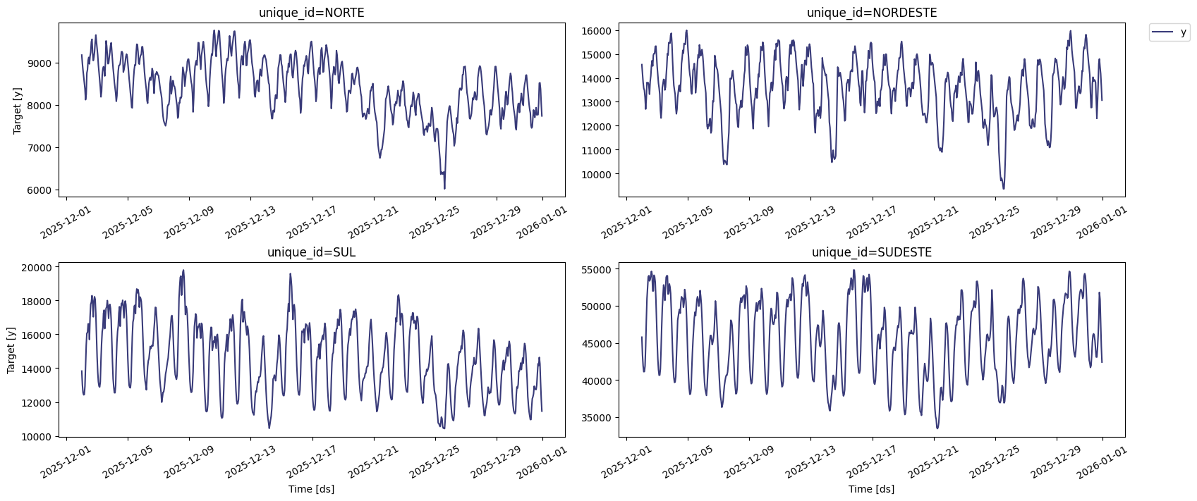
TimeGPT includes convenient plotting capabilities.
# Plotting the time series data
nixtla_client.plot(
    df_ons_se,               # The DataFrame containing the time series data
    max_insample_length=720  # Maximum number of data points to plot for the in-sample period
)
Even if your dataset’s column names don’t match TimeGPT’s default expectations, you can still utilize it by explicitly defining the correct column mappings.
nixtla_client.plot(
  df,
  time_col = 'Date',
  id_col = 'Store',
  target_col = 'Weekly_Sales'
)
For instance, in the example above, time_col designates the timestamp column as ‘Date’, id_col identifies the series by ‘Store’, and target_col specifies the observed values as ‘Weekly_Sales’. When these parameters are omitted, TimeGPT automatically searches for columns named ds, unique_id, and y.
🔮 Splitting and forecasting over the test set
'''
The test dataset is constructed by extracting the final 96 observations (equivalent to 4 days)
for each distinct time (or subsystem).
'''
test_df = df_ons_se.groupby('unique_id').tail(96)

'''
Subsequently, the training input data is formed by isolating the 21-day period immediately preceding the test set,
thereby excluding the test observations.
'''
input_df = df_ons_se.groupby('unique_id').apply(lambda group: group.iloc[-1104:-96]).reset_index(drop=True)
/tmp/ipykernel_25303/3361290161.py:11: DeprecationWarning: DataFrameGroupBy.apply operated on the grouping columns. This behavior is deprecated, and in a future version of pandas the grouping columns will be excluded from the operation. Either pass `include_groups=False` to exclude the groupings or explicitly select the grouping columns after groupby to silence this warning.
  input_df = df_ons_se.groupby('unique_id').apply(lambda group: group.iloc[-1104:-96]).reset_index(drop=True)
💡 Zero-shot Forecasting
Zero-shot forecasting represents a pivotal advancement in predictive analytics, enabling a model to generate accurate predictions for time series data without explicit prior training on that specific series. Drawing parallels to the broader concept of zero-shot learning in artificial intelligence, this methodology leverages a foundational model’s extensive pre-trained knowledge base to generalize intricate patterns, trends, and seasonalities across diverse datasets.
In the context of TimeGPT, this entails utilizing its inherent understanding of temporal dynamics, acquired from vast quantities of historical time series, to infer future values for an entirely novel or previously unseen series. This approach is particularly advantageous in scenarios where the acquisition of sufficient historical data for traditional model training is impractical, or where rapid deployment of predictive capabilities is paramount for emerging data streams.
For the current analysis of Brazilian electricity demand, TimeGPT’s zero-shot capability offers a robust initial forecasting benchmark. By supplying the input data to the pre-trained TimeGPT model, it can immediately generate forecasts for the hourly load curve across various regional subsystems without requiring any bespoke fine-tuning.
In this specific context, the nixtla_client.forecast function is utilized with its basic configuration to demonstrate this zero-shot predictive capability.
While providing a swift and accessible predictive baseline, the efficacy of zero-shot forecasting can vary depending on the complexity and unique characteristics of the target time series.
Subsequent fine-tuning steps often enhance performance by adapting the foundational model to the subtle nuances of the specific dataset, as will be demonstrated in further sections.
# Generates predictions using the Nixtla Client for zero-shot forecasting.
zeroshot_fcst = nixtla_client.forecast(
     df = input_df,                   # The input DataFrame containing the training data.
     h  = 96,                         # The forecast horizon, specifying the number of future time steps to predict.
     level = [90],                    # The confidence level(s) for the prediction intervals, e.g., 90% for a 90% confidence band.
)
WARNING:nixtla.nixtla_client:The specified horizon "h" exceeds the model horizon, this may lead to less accurate forecasts. Please consider using a smaller horizon.
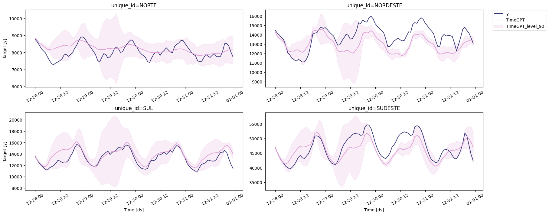
🔍 Visualizing Forecast Results
The figure below displays the predictions generated by TimeGPT for each series.
# Plots the forecasts generated by TimeGPT.
nixtla_client.plot(
    test_df,            # The DataFrame containing the actual test data for comparison.
    zeroshot_fcst,      # The DataFrame containing the generated forecasts.
    models=['TimeGPT'], # Specifies the forecasting model(s) to be displayed.
    level=[90]          # The confidence level(s) for the prediction intervals, if included in the forecast.
)
🛠️ Fine-tuning TimeGPT
The finetune_steps parameter governs the number of training iterations applied to TimeGPT, where each step involves updating the model’s internal parameters subsequent to the processing of a data batch. This mechanism allows for targeted adaptation of the model to specific datasets.
While fine-tuning is frequently employed to enhance predictive performance, its efficacy is not universally guaranteed. Excessive fine-tuning steps can lead to model overfitting, wherein the model’s capacity for generalization to unseen data is compromised, resulting in suboptimal predictive accuracy. Furthermore, increasing the number of fine-tuning steps inherently incurs greater computational overhead, extending the time required for model training and inference.
A pragmatic approach involves commencing with a modest value for finetune_steps, such as 10. This initial setting can then be iteratively adjusted upwards, systematically evaluating its impact on the model’s performance against a dedicated validation set to identify an optimal balance between adaptability and generalization.
finetune_loss parameter, which takes any values in MAE, MSE, RMSE, MAPE, sMAPE. The loss function directs the training of the model during fine-tuning.
| Loss function | Characteristics |
|---|---|
| Mean absolute error (mae) | • Robust to outliers • Penalizes all errors equally • Same units as data |
| Mean squared error (mse) | • Heavier penalty for large errors • Sensitive to outliers • Not the same units as data |
| Root mean squared error (rmse) | • Same units as data • Heavier penalty for large errors |
| Mean absolute percentage error (mape) | • Expressed as a percentage • Heavier penalty on positive errors • Avoid if data points are close or equal to 0. |
| Symmetric mean absolute percentage error (smape) | • Expressed as a percentage • Equal penalty for positive and negative errors • Avoid if data points are close or equal to 0. |
Source: Peixeiro, M. (2025)
# Generates predictions using the Nixtla Client.
finetune_fcst = nixtla_client.forecast(
     df = input_df,                   # The input DataFrame containing the training data for fine-tuning.
     h  = 96,                         # The forecast horizon, specifying the number of future time steps to predict (e.g., 96 steps ahead).
     level = [90],                    # The confidence level(s) for the prediction intervals, e.g., 90% for a 90% confidence band.
     finetune_steps = 10,             # Sets the number of steps for fine-tuning
     finetune_loss = 'mae',           # [Optional] Sets the loss function to be used during fine-tuning (e.g., Mean Absolute Error).
     model = 'timegpt-1-long-horizon' # Specifies the TimeGPT model architecture, such as 'timegpt-1-long-horizon' for extended forecasting capabilities.
)
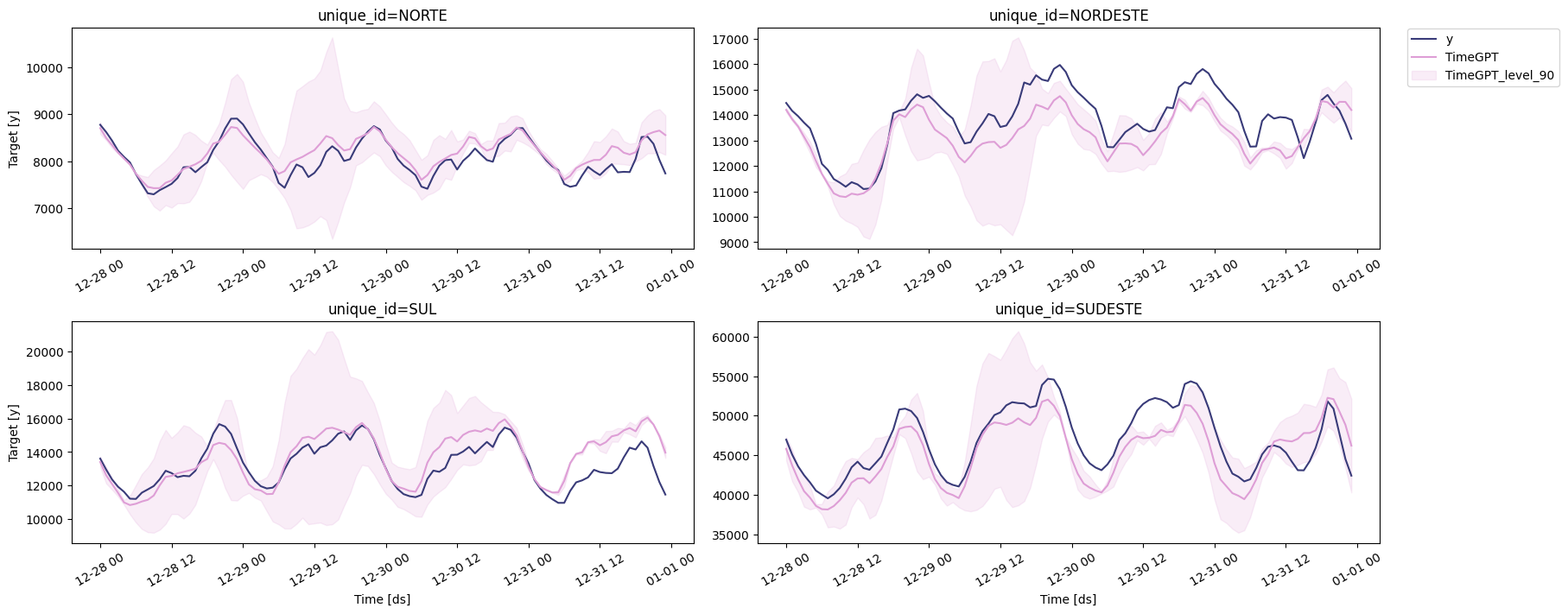
🔍 Visualizing Fine-tuned Results
The figure below displays the predictions generated by the fine-tuned model for each series.
# Plots the forecasts generated by TimeGPT.
nixtla_client.plot(
    test_df,            # The DataFrame containing the actual test data for comparison.
    finetune_fcst,      # The DataFrame containing the generated forecasts.
    models=['TimeGPT'], # Specifies the forecasting model(s) to be displayed.
    level=[90]          # The confidence level(s) for the prediction intervals, if included in the forecast.
)
TimeGPT automatically deduced the underlying data frequency from the provided timestamps and subsequently generated predictions for each individual time series. However, it did not engage in multivariate forecasting, meaning it did not leverage data from one subsystem (e.g., Southeast/Midwest) to inform predictions for another (e.g., Northeast). Instead, the model processed and forecasted each series independently.
Consequently, this approach may overlook potential interdependencies among the series, which could otherwise contribute to more accurate predictive outcomes.
🏅 Performance Evaluation
'''
To preempt potential column conflicts arising from subsequent merge operations,
a duplicate of the original test DataFrame is created.
'''
eval_df = test_df.copy()

'''
The 'ds' column within the forecast DataFrame is converted to a datetime object
to ensure appropriate temporal data handling.
'''
zeroshot_fcst['ds'] = pd.to_datetime(finetune_fcst['ds'])

finetune_fcst['ds'] = pd.to_datetime(finetune_fcst['ds'])
finetune_fcst.rename(columns={'TimeGPT': 'TimeGPT-finetuned'}, inplace=True)

'''
The generated predictions are subsequently merged with the test dataset
based on the common identifiers ('unique_id' and 'ds').
'''
eval_df = pd.merge(eval_df, finetune_fcst, 'left', ['unique_id', 'ds'])
eval_df = pd.merge(eval_df, zeroshot_fcst, 'left', ['unique_id', 'ds'])

'''
The forecast performance is rigorously assessed using Mean Absolute Error (MAE),
and Symmetric Mean Absolute Percentage Error (SMAPE) as key evaluation metrics.
'''
evaluation = evaluate(
    eval_df,                                 # This DataFrame encompasses both the actual observations and the corresponding predictions.
    metrics=[mae, smape],                    # The quantitative measures employed for performance assessment.
    models=['TimeGPT', 'TimeGPT-finetuned'], # Specifies the forecasting model(s) for which evaluation is being performed.
    target_col="y",                          # Identifies the column containing the true observed values.
    id_col='unique_id'                       # Denotes the column that uniquely identifies each individual time series.
).round(2)

evaluation
| unique_id | metric | TimeGPT | TimeGPT-finetuned | |
|---|---|---|---|---|
| 0 | NORDESTE | mae | 1092.04 | 761.11 |
| 1 | NORTE | mae | 290.03 | 167.59 |
| 2 | SUDESTE | mae | 2440.69 | 2314.41 |
| 3 | SUL | mae | 676.29 | 744.11 |
| 4 | NORDESTE | smape | 0.04 | 0.03 |
| 5 | NORTE | smape | 0.02 | 0.01 |
| 6 | SUDESTE | smape | 0.03 | 0.03 |
| 7 | SUL | smape | 0.03 | 0.03 |
A more granular examination of the evaluation metrics across individual subsystems reveals nuanced performance variations. For the Northeast (NORDESTE) subsystem, the fine-tuned TimeGPT model demonstrated a considerable improvement in Mean Absolute Error (MAE), decreasing from 1092.06 to 761.11. Similarly, its symmetric Mean Absolute Percentage Error (sMAPE) also saw a reduction from 0.04 to 0.03. The Northern (NORTE) subsystem experienced the most significant enhancement through fine-tuning, with MAE dropping from 290.03 to 167.59 and sMAPE halving from 0.02 to 0.01. These improvements indicate that fine-tuning was particularly effective in optimizing predictions for these regions.
Conversely, the Southeast (SUDESTE) subsystem, which exhibits the highest absolute load values, presented a more modest improvement in MAE, decreasing from 2440.69 to 2314.41. Its sMAPE, however, remained consistent at 0.03 for both models. This suggests that while fine-tuning offered some benefit, the inherent scale and potential complexity of the Southeast’s load curve still pose a substantial challenge for both model configurations. Interestingly, for the Southern (SUL) subsystem, the fine-tuned model exhibited a slight increase in MAE (from 676.29 to 744.11), although its sMAPE remained unchanged at 0.03. This localized degradation in MAE, despite a stable sMAPE, warrants further investigation into the specific characteristics of the SUL data that might have led to this outcome.
In summary, fine-tuning generally yielded beneficial outcomes, particularly for the NORDESTE and NORTE regions, where prediction accuracy saw notable improvements. The SUDESTE subsystem, despite some enhancement, continues to represent the most challenging forecasting task in terms of absolute error. The slight deterioration in MAE for SUL underscores the importance of subsystem-specific analysis, as model optimizations may not uniformly translate to improved performance across all distinct time series within a heterogeneous dataset.
'''
The mean of the evaluation metrics across all time series is computed for the TimeGPT model.
'''
average_metrics = evaluation.groupby('metric')[['TimeGPT', 'TimeGPT-finetuned']].mean().round(2)

average_metrics
| TimeGPT | TimeGPT-finetuned | |
|---|---|---|
| metric | ||
| mae | 1124.74 | 996.80 |
| smape | 0.03 | 0.02 |
From the evaluation, the zero-shot TimeGPT model exhibited an average Mean Absolute Error (MAE) of approximately 1124.74 MWmed and a symmetric Mean Absolute Percentage Error (sMAPE) of 0.03% across all subsystems. Following fine-tuning, the TimeGPT-finetuned model demonstrated improved performance, achieving an average MAE of 996.80 MWmed and an sMAPE of 0.02%.
While the MAE values appear substantial, this is primarily attributable to the scale of the data, which is expressed in MWmed. Consequently, the sMAPE offers a more intuitively interpretable measure of forecast accuracy in this context, indicating an average deviation of 0.02% for the fine-tuned model when forecasting the subsequent 4-day load curve across the four distinct subsystems. This enhanced level of performance was achieved through fine-tuning, notably without the incorporation of exogenous variables into the model.
🤿 Controling the depth of fine-tuning
Beyond the specification of fine-tuning steps and the chosen loss metric, the finetune_depth argument provides a mechanism to modulate the extent of parameter adjustment within the TimeGPT model. This parameter accepts integer values ranging from 1 to 5, where a value of 1 corresponds to the fine-tuning of a limited subset of parameters, while a value of 5 indicates the adjustment of all available model parameters. A notable limitation, however, is the absence of detailed disclosure regarding the precise number of parameters fine-tuned at each depth level within the official documentation.
It is crucial to recognize that an increment in finetune_depth directly correlates with an increased computational burden, leading to longer prediction generation times. This is attributable to the more extensive parameter tuning required for larger depth values. Furthermore, judicious selection of this parameter is essential, as elevated values for both finetune_steps and finetune_depth collectively heighten the risk of model overfitting. Overfitting, in this context, would compromise the model’s generalization capabilities, potentially yielding suboptimal forecasting performance on unseen data. Consequently, a recommended practice involves an incremental increase of the finetune_depth parameter, coupled with rigorous monitoring of the model’s performance on a dedicated validation set to identify an optimal configuration.
# Re-initialize eval_df to its state before finetune_depth_fcst was merged.
# This ensures that eval_df contains 'y', 'TimeGPT', and 'TimeGPT-finetuned'
# (and their prediction intervals if present), but not 'TimeGPT-finetuned-depth' yet.
# We use the globally available 'test_df', 'finetune_fcst', and 'zeroshot_fcst'.

temp_eval_df = test_df.copy()

# Ensure 'ds' columns are datetime objects before merging, as they might have been converted earlier.
# Using copies to avoid modifying original global DataFrames in case they are used elsewhere.
finetune_fcst_for_merge = finetune_fcst.copy()
zeroshot_fcst_for_merge = zeroshot_fcst.copy()
finetune_fcst_for_merge['ds'] = pd.to_datetime(finetune_fcst_for_merge['ds'])
zeroshot_fcst_for_merge['ds'] = pd.to_datetime(zeroshot_fcst_for_merge['ds'])

# Merge previously computed forecasts (TimeGPT-finetuned and TimeGPT) into the temporary eval_df.
# This recreates the state of eval_df as it should be before this cell's specific additions.
temp_eval_df = pd.merge(temp_eval_df, finetune_fcst_for_merge, 'left', ['unique_id', 'ds'])
temp_eval_df = pd.merge(temp_eval_df, zeroshot_fcst_for_merge, 'left', ['unique_id', 'ds'])

# Original code for finetune_depth_fcst
finetune_depth_fcst = nixtla_client.forecast(
    df = input_df,
    h = 96,
    finetune_steps = 10,
    finetune_depth = 2,
    finetune_loss = 'mae',
    model = 'timegpt-1-long-horizon'
)

finetune_depth_fcst.rename(columns={"TimeGPT": "TimeGPT-finetuned-depth"},
inplace=True)

# Ensure 'ds' column is datetime for finetune_depth_fcst before merging
finetune_depth_fcst['ds'] = pd.to_datetime(finetune_depth_fcst['ds'])

# Now merge the new finetune_depth_fcst into the correctly initialized temp_eval_df
eval_df = pd.merge(temp_eval_df, finetune_depth_fcst, 'left', ['unique_id', 'ds'])

evaluation_depth = evaluate(
    eval_df,
    metrics=[mae, smape],
    models=['TimeGPT', 'TimeGPT-finetuned', 'TimeGPT-finetuned-depth'],
    target_col='y',
    id_col='unique_id'
).round(2)

'''
The mean of the evaluation metrics across all time series is computed for the TimeGPT model.
'''
average_metrics_depth = evaluation_depth.groupby('metric')[['TimeGPT', 'TimeGPT-finetuned', 'TimeGPT-finetuned-depth']].mean().round(2)

average_metrics_depth
| TimeGPT | TimeGPT-finetuned | TimeGPT-finetuned-depth | |
|---|---|---|---|
| metric | |||
| mae | 1124.76 | 996.80 | 1094.26 |
| smape | 0.03 | 0.02 | 0.02 |
A comparative analysis of the average_metrics_depth reveals nuanced insights into the impact of fine-tuning depth on model performance. The baseline TimeGPT model recorded an average Mean Absolute Error (MAE) of 1124.76 and a Symmetric Mean Absolute Percentage Error (sMAPE) of 0.03. The initial fine-tuning, without explicit depth specification (TimeGPT-finetuned), notably improved these metrics, achieving an MAE of 996.80 and an sMAPE of 0.02.
However, the introduction of a finetune_depth of 2 (TimeGPT-finetuned-depth) resulted in a slight degradation of performance compared to the standard fine-tuned model, with its MAE increasing to 1094.26 and sMAPE of 0.02. Interestingly, the TimeGPT-finetuned-depth model even surpassed the baseline TimeGPT in terms of MAE, indicating that this particular depth setting did not yield beneficial outcomes in this context. This suggests that while fine-tuning can enhance predictive accuracy, the specific finetune_depth parameter requires careful optimization, as an arbitrary setting may lead to suboptimal or even regressed performance.
⚖️ Pros and cons of TimeGPT (foundation) forecasting model
Advantages:
- Ease and Speed of Use: Accessing TimeGPT through its API significantly streamlines the forecasting process, requiring minimal code and setup. This facilitates rapid model interaction, eliminating the need for local environment configuration.
- Comprehensive Native Functions: The model is equipped with a rich set of built-in functionalities, allowing users to perform complex forecasting tasks efficiently without extensive custom coding.
- Platform Independence: TimeGPT’s cloud-based nature ensures consistent performance across various devices, irrespective of local hardware specifications.
- Potential for Free Access: Free tiers or trial periods may be available, enabling users to explore the model’s capabilities before committing to a paid subscription.
Disadvantages:
- Subscription-Based Model: While initial testing might be free, sustained use often requires a paid subscription, which may not be feasible for all individuals or organizations.
- Service Availability: The model’s accessibility is contingent on server status; service interruptions or downtime could temporarily hinder its use.
Recommended Use Cases:
TimeGPT is particularly well-suited for:
- Forecasting across diverse time horizons (long and short) with the incorporation of exogenous features.
- Fine-tuning models in scenarios where local computational resources are limited.
📚 References
Awan, A. A. (2024). Time Series Forecasting With TimeGPT.
Barbosa Filho, L. H. Prevendo Demanda de Energia Usando TimeGPT no Python.
Peixeiro, M. (2025). Time Series Forecasting Using Foundation Models.
Peixeiro, M. (2025). TimeSeriesForecastingUsingFoundationModels, GitHub repository.